Forecasting Market Movements Using Tensorflow - Intro into Machine Learning for Finance (Part 2)


Here is a full script used in this article.
Multi-Layer Perceptron for Classification
Is it possible to create a neural network for predicting daily market movements from a set of standard trading indicators?
In this post we’ll be looking at a simple model using Tensorflow to create a framework for testing and development, along with some preliminary results and suggested improvements.
The ML Task and Input Features
To keep the basic design simple, it’s setup for a binary classification task, predicting whether the next day’s close is going to be higher or lower than the current, corresponding to a prediction to either go long or short for the next time period. In reality, this could be applied to a bot which calculates and executes a set of positions at the start of a trading day to capture the day’s movement.
The model is currently using 4 input features (again, for simplicity): 15 + 50 day RSI and 14 day Stochastic K and D.
These were chosen due to the indicators being normalized between 0 and 100, meaning that the underlying price of the asset is of no concern to the model, allowing for greater generalization.
While it would be possible to train the model against any number of other trading indicators or otherwise, I’d recommend sticking to those that are either normalized by design or could be modified to be price or volatility normalized. Otherwise a single model is unlikely to work on a range of stocks.
Dataset Generation
The dataset generation and neural network scripts have been split into two distinct modules to allow for both easier modification, and the ability to re-generate the full datasets only when necessary — as it takes a long time.
Currently the generator script is setup with a list of S&P 500 stocks to download daily candles since 2015 and process them into the required trading indicators, which will be used as the input features of the model.
Everything is then split into a set of training data (Jan 2015 — June 2017) and evaluation data (June 2017 — June 2018) and written as CSVs to “train” and “eval” folders in the directory that the script was run.
These files can then be read on demand by the ML script to train and evaluate the model without the need to re-download and process any more data.
Model Training
At start-up, the script reads all the CSV files in the “train” and “eval” folders into arrays of data for use throughout the training process. With such a small dataset, the RAM requirements will be low enough not to warrant extra complexity. But, for a significantly larger dataset, this would have to be updated to only read a sample of the full data at a time, rotating the data held in memory every few thousand training steps. This would, however, come at the cost of greater disk IO, slowing down training.
The neural network itself is also extremely small, as testing showed that with larger networks, evaluation accuracies tended to diverge quickly.
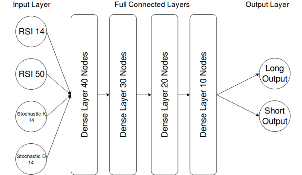
The network “long Output” and “short Output” are used as a binary predictor, with the highest confidence value being used as the model prediction for the coming day.
The “dense” layers within the architecture mean that each neuron is connected to the outputs of all the neurons in the layer below. These neurons are the same as described in “Intro into Machine Learning for Finance (Part 1)”, and use tanh as the activation function, which is a common choice for a small neural network.
 Yoshi Yokokawa
Some types of data and networks can work better with different activation functions, such RELU or ELU for deeper networks. RELU (Rectifier Linear Unit) attempts to solve the vanishing gradient problem in deeper architectures, and the ELU is a variation on this to make training yet more efficient.
TensorBoard
As well as displaying prediction accuracy stats in the terminal every 1000 training steps, the ML script is also setup to record summaries for use with TensorBoard — making graphing of the training process much easier.
While I haven’t included anything other than scalar summaries, it’s possible to record everything from histograms of the node weightings to sample images or audio from the training data.
To use TensorBoard with the saved summaries, simply set the — logdir flag to directory you’re running the ML script in. You then open the browser of your choice and enter “localhost:6006” into the search bar. All being well, you now have a set of auto-updating charts.
Training results
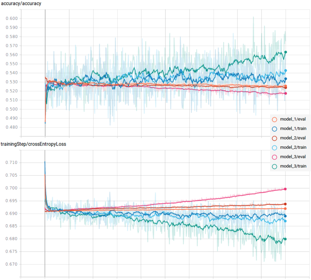
The results were, as expected, less than spectacular due to the simplicity of the example design and its input features.
We can see clear overfitting, as the loss/ error increases against the evaluation dataset for all tests, especially so on the larger networks. This means that the network is only learning the pattern of the specific training samples, rather than an a more generalized model. On top of this, the training accuracies aren’t amazingly high — only achieving a few percent above completely random guesses.
Suggestions for Modification and Improvement
The example code provides a nice model that can be played around with to help understand how everything works — but it serves more as a starting framework than a working model for prediction. As such, a few suggestions for improvements that you might want to make and ideas you could test
Input features
In its current state, the dataset is generated with only 4 input features and the model only looks at one point in time. This severely limits what you can expect it to be able to learn — would you be able to trade only looking at a few indicator values for one day in isolation?
First, modifying the dataset generation script to calculate more trading indicators and save them to the CSV. TA-lib has a wide range of functions which can be found here.
I recommend sticking to normalized indicators, similar to Stoch and RSI, as this takes the relative price of the asset out of the equation, so that the model can be generalized across a range of stocks rather than needing a different model for each.
Next, you could modify the ML script to read the last 10 data periods as the input at each time step, rather than just the one. This allows it to start learning more complex convergence and divergence patterns in the oscillators over time.
Network Architecture
As mentioned earlier, the network is tiny due to the lack of data and feature complexity of the example task. This will have to be altered to accommodate the extra data being fed by the added indicators.
The easiest way to do this would be to change the node layout variable to add extra layers or greater numbers of neurons per layer. You may also wish to experiment with different types of layer other than fully connected. Convolutional layers are often used for pattern recognition tasks with images, so could be interesting to test out on financial chart data.
Dataset labels
The dataset is labeled at “long” if price difference is >=0, otherwise “short”. However, you may wish to change the threshold to be equal to the median price change over the length of the data, to give a more balanced set of training data.
You may even wish to add a third category of “neutral” for days where the price stays within a limited range.
On top of this, the script also has the ability to vary the look ahead period for the increase or decrease in price. So it could be tested with a longer term prediction.
Conclusion
With the implementation of the suggested improvements, it is certainly possible to improve on the model to the point where it could be used as a complimentary trading indicator to a standard rule based strategy.
However, expectations should be tempered when it comes to such a simple architecture and training task. Machine learning can really set itself apart with a more refined network structure and prediction task.
As such, in the next article we’ll be looking at Supervised, Unsupervised and Reinforcement Learning, and how they can be used to create time series predictor and to analyze relationships in data to help refine strategies.
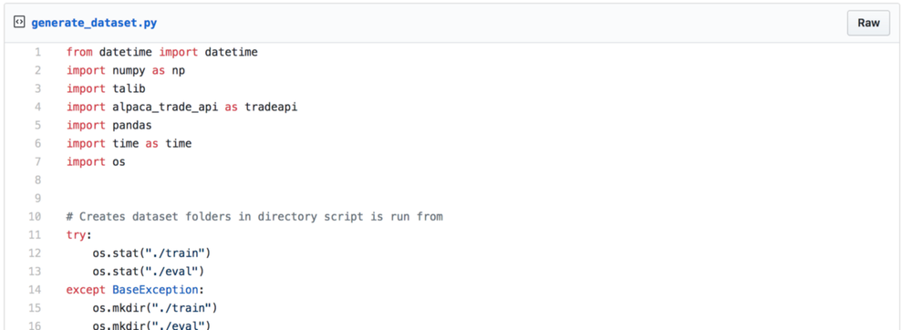
Full Script
from datetime import datetime
import numpy as np
import talib
import alpaca_trade_api as tradeapi
import pandas
import time as time
import os
# Creates dataset folders in directory script is run from
try:
os.stat("./train")
os.stat("./eval")
except BaseException:
os.mkdir("./train")
os.mkdir("./eval")
# api = tradeapi.REST(key_id= < your key id >, secret_key= < your secret
# key > )
barTimeframe = "1D" # 1Min, 5Min, 15Min, 1H, 1D
assetList = np.loadtxt(
"assetList.txt",
comments="#",
delimiter=",",
unpack=False,
dtype="str")
# ISO8601 date format
trainStartDate = "2015-01-01T00:00:00.000Z"
trainEndDate = "2017-06-01T00:00:00.000Z"
evalStartDate = "2017-06-01T00:00:00.000Z"
evalEndDate = "2018-06-01T00:00:00.000Z"
targetLookaheadPeriod = 1
startCutoffPeriod = 50 # Set to length of maximum period indicator
# Tracks position in list of symbols to download
iteratorPos = 0
assetListLen = len(assetList)
while iteratorPos < assetListLen:
try:
symbol = assetList[iteratorPos]
# Returns market data as a pandas dataframe
returned_data = api.get_bars(
symbol,
barTimeframe,
start_dt=trainStartDate,
end_dt=evalEndDate).df
# Processes all data into numpy arrays for use by talib
timeList = np.array(returned_data.index)
openList = np.array(returned_data.open, dtype=np.float64)
highList = np.array(returned_data.high, dtype=np.float64)
lowList = np.array(returned_data.low, dtype=np.float64)
closeList = np.array(returned_data.close, dtype=np.float64)
volumeList = np.array(returned_data.volume, dtype=np.float64)
# Adjusts data lists due to the reward function look ahead period
shiftedTimeList = timeList[:-targetLookaheadPeriod]
shiftedClose = closeList[targetLookaheadPeriod:]
highList = highList[:-targetLookaheadPeriod]
lowList = lowList[:-targetLookaheadPeriod]
closeList = closeList[:-targetLookaheadPeriod]
# Calculate trading indicators
RSI14 = talib.RSI(closeList, 14)
RSI50 = talib.RSI(closeList, 50)
STOCH14K, STOCH14D = talib.STOCH(
highList, lowList, closeList, fastk_period=14, slowk_period=3, slowd_period=3)
# Calulate network target/ reward function for training
closeDifference = shiftedClose - closeList
closeDifferenceLen = len(closeDifference)
# Creates a binary output if the market moves up or down, for use as
# one-hot labels
longOutput = np.zeros(closeDifferenceLen)
longOutput[closeDifference >= 0] = 1
shortOutput = np.zeros(closeDifferenceLen)
shortOutput[closeDifference < 0] = 1
# Constructs the dataframe and writes to CSV file
outputDF = {
"close": closeList, # Not to be included in network training, only for later analysis
"RSI14": RSI14,
"RSI50": RSI50,
"STOCH14K": STOCH14K,
"STOCH14D": STOCH14D,
"longOutput": longOutput,
"shortOutput": shortOutput
}
# Makes sure the dataframe columns don't get mixed up
columnOrder = ["close", "RSI14", "RSI50", "STOCH14K",
"STOCH14D", "longOutput", "shortOutput"]
outputDF = pandas.DataFrame(
data=outputDF,
index=shiftedTimeList,
columns=columnOrder)[
startCutoffPeriod:]
# Splits data into training and evaluation sets
trainingDF = outputDF[outputDF.index < evalStartDate]
evalDF = outputDF[outputDF.index >= evalStartDate]
if (len(trainingDF) > 0 and len(evalDF) > 0):
print("writing " + str(symbol) +
", data len: " + str(len(closeList)))
trainingDF.to_csv("./train/" + symbol + ".csv", index_label="date")
evalDF.to_csv("./eval/" + symbol + ".csv", index_label="date")
except BaseException:
pass
time.sleep(5) # To avoid API rate limits
iteratorPos += 1from datetime import datetime
import numpy as np
import talib
import alpaca_trade_api as tradeapi
import pandas
import time as time
import os
# Creates dataset folders in directory script is run from
try:
os.stat("./train")
os.stat("./eval")
except BaseException:
os.mkdir("./train")
os.mkdir("./eval")
# api = tradeapi.REST(key_id= < your key id >, secret_key= < your secret
# key > )
barTimeframe = "1D" # 1Min, 5Min, 15Min, 1H, 1D
assetList = np.loadtxt(
"assetList.txt",
comments="#",
delimiter=",",
unpack=False,
dtype="str")
# ISO8601 date format
trainStartDate = "2015-01-01T00:00:00.000Z"
trainEndDate = "2017-06-01T00:00:00.000Z"
evalStartDate = "2017-06-01T00:00:00.000Z"
evalEndDate = "2018-06-01T00:00:00.000Z"
targetLookaheadPeriod = 1
startCutoffPeriod = 50 # Set to length of maximum period indicator
# Tracks position in list of symbols to download
iteratorPos = 0
assetListLen = len(assetList)
while iteratorPos < assetListLen:
try:
symbol = assetList[iteratorPos]
# Returns market data as a pandas dataframe
returned_data = api.get_bars(
symbol,
barTimeframe,
start_dt=trainStartDate,
end_dt=evalEndDate).df
# Processes all data into numpy arrays for use by talib
timeList = np.array(returned_data.index)
openList = np.array(returned_data.open, dtype=np.float64)
highList = np.array(returned_data.high, dtype=np.float64)
lowList = np.array(returned_data.low, dtype=np.float64)
closeList = np.array(returned_data.close, dtype=np.float64)
volumeList = np.array(returned_data.volume, dtype=np.float64)
# Adjusts data lists due to the reward function look ahead period
shiftedTimeList = timeList[:-targetLookaheadPeriod]
shiftedClose = closeList[targetLookaheadPeriod:]
highList = highList[:-targetLookaheadPeriod]
lowList = lowList[:-targetLookaheadPeriod]
closeList = closeList[:-targetLookaheadPeriod]
# Calculate trading indicators
RSI14 = talib.RSI(closeList, 14)
RSI50 = talib.RSI(closeList, 50)
STOCH14K, STOCH14D = talib.STOCH(
highList, lowList, closeList, fastk_period=14, slowk_period=3, slowd_period=3)
# Calulate network target/ reward function for training
closeDifference = shiftedClose - closeList
closeDifferenceLen = len(closeDifference)
# Creates a binary output if the market moves up or down, for use as
# one-hot labels
longOutput = np.zeros(closeDifferenceLen)
longOutput[closeDifference >= 0] = 1
shortOutput = np.zeros(closeDifferenceLen)
shortOutput[closeDifference < 0] = 1
# Constructs the dataframe and writes to CSV file
outputDF = {
"close": closeList, # Not to be included in network training, only for later analysis
"RSI14": RSI14,
"RSI50": RSI50,
"STOCH14K": STOCH14K,
"STOCH14D": STOCH14D,
"longOutput": longOutput,
"shortOutput": shortOutput
}
# Makes sure the dataframe columns don't get mixed up
columnOrder = ["close", "RSI14", "RSI50", "STOCH14K",
"STOCH14D", "longOutput", "shortOutput"]
outputDF = pandas.DataFrame(
data=outputDF,
index=shiftedTimeList,
columns=columnOrder)[
startCutoffPeriod:]
# Splits data into training and evaluation sets
trainingDF = outputDF[outputDF.index < evalStartDate]
evalDF = outputDF[outputDF.index >= evalStartDate]
if (len(trainingDF) > 0 and len(evalDF) > 0):
print("writing " + str(symbol) +
", data len: " + str(len(closeList)))
trainingDF.to_csv("./train/" + symbol + ".csv", index_label="date")
evalDF.to_csv("./eval/" + symbol + ".csv", index_label="date")
except BaseException:
pass
time.sleep(5) # To avoid API rate limits
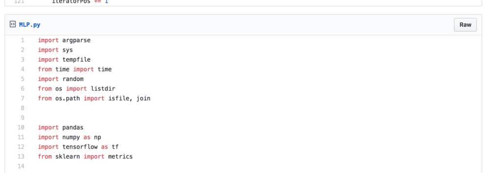
iteratorPos += 1import argparse
import sys
import tempfile
from time import time
import random
from os import listdir
from os.path import isfile, join
import pandas
import numpy as np
import tensorflow as tf
from sklearn import metrics
# model settings
# Static seed to allow for reproducability between training runs
tf.set_random_seed(12345)
trainingCycles = 500000 # Number of training steps before ending
batchSize = 1000 # Number of examples per training batch
summarySteps = 1000 # Number of training steps between each summary
dropout = 0.5 # Node dropout for training
nodeLayout = [40, 30, 20, 10] # Layout of nodes in each layer
mainDirectory = str("./model_1/")
trainFiles = [f for f in listdir("./train/") if isfile(join("./train/", f))]
evalFiles = [f for f in listdir("./eval/") if isfile(join("./eval/", f))]
# Initialises data arrays
trainDataX = np.empty([0, 4])
trainDataY = np.empty([0, 2])
evalDataX = np.empty([0, 4])
evalDataY = np.empty([0, 2])
# Reads training data into memory
readPos = 0
for fileName in trainFiles:
importedData = pandas.read_csv("./train/" + fileName, sep=',')
xValuesDF = importedData[["RSI14", "RSI50", "STOCH14K", "STOCH14D"]]
yValuesDF = importedData[["longOutput", "shortOutput"]]
xValues = np.array(xValuesDF.values.tolist())
yValues = np.array(yValuesDF.values.tolist())
trainDataX = np.concatenate([trainDataX, xValues], axis=0)
trainDataY = np.concatenate([trainDataY, yValues], axis=0)
if readPos % 50 == 0 and readPos > 0:
print("Loaded " + str(readPos) + " training files")
readPos += 1
print("\n\n")
# Reads evalutation data into memory
readPos = 0
for fileName in evalFiles:
importedData = pandas.read_csv("./eval/" + fileName, sep=',')
xValuesDF = importedData[["RSI14", "RSI50", "STOCH14K", "STOCH14D"]]
yValuesDF = importedData[["longOutput", "shortOutput"]]
xValues = np.array(xValuesDF.values.tolist())
yValues = np.array(yValuesDF.values.tolist())
evalDataX = np.concatenate([evalDataX, xValues], axis=0)
evalDataY = np.concatenate([evalDataY, yValues], axis=0)
if readPos % 50 == 0 and readPos > 0:
print("Loaded " + str(readPos) + " training files")
readPos += 1
print("\n\n")
# used to sample batches from your data for training
def createTrainingBatch(amount):
randomBatchPos = np.random.randint(0, trainDataX.shape[0], amount)
xOut = trainDataX[randomBatchPos]
yOut = trainDataY[randomBatchPos]
return xOut, yOut
tf.logging.set_verbosity(tf.logging.INFO)
# ML training and evaluation functions
def train():
globalStepTensor = tf.Variable(0, trainable=False, name='global_step')
sess = tf.InteractiveSession()
# placeholder for the input features
x = tf.placeholder(tf.float32, [None, 4])
# placeholder for the one-hot labels
y = tf.placeholder(tf.float32, [None, 2])
# placeholder for node dropout rate
internalDropout = tf.placeholder(tf.float32, None)
net = x # input layer is the trading indicators
# Creates the neural network model
with tf.name_scope('network'):
# Initialises each layer in the network
layerPos = 0
for units in nodeLayout:
net = tf.layers.dense(
net,
units=units,
activation=tf.nn.tanh,
name=str(
"dense" +
str(units) +
"_" +
str(layerPos))) # adds each layer to the networm as specified by nodeLayout
# dropout layer after each layer
net = tf.layers.dropout(net, rate=internalDropout)
layerPos += 1
logits = tf.layers.dense(
net, 2, activation=tf.nn.softmax) # network output
with tf.name_scope('lossFunction'):
cross_entropy_loss = tf.reduce_mean(
tf.nn.softmax_cross_entropy_with_logits_v2(
labels=y,
logits=logits)) # on NO account put this within a name scope - tensorboard shits itself
with tf.name_scope('trainingStep'):
tf.summary.scalar('crossEntropyLoss', cross_entropy_loss)
trainStep = tf.train.AdamOptimizer(0.0001).minimize(
cross_entropy_loss, global_step=globalStepTensor)
with tf.name_scope('accuracy'):
correctPrediction = tf.equal(tf.argmax(logits, 1), tf.argmax(y, 1))
accuracy = tf.reduce_mean(tf.cast(correctPrediction, tf.float32))
tf.summary.scalar('accuracy', accuracy)
merged = tf.summary.merge_all()
trainWriter = tf.summary.FileWriter(
mainDirectory + '/train', sess.graph, flush_secs=1, max_queue=2)
evalWriter = tf.summary.FileWriter(
mainDirectory + '/eval', sess.graph, flush_secs=1, max_queue=2)
tf.global_variables_initializer().run()
# Saves the model at defined checkpoints and loads any available model at
# start-up
saver = tf.train.Saver(max_to_keep=2, name="checkpoint")
path = tf.train.get_checkpoint_state(mainDirectory)
if path is not None:
saver.restore(sess, tf.train.latest_checkpoint(mainDirectory))
lastTime = time()
while tf.train.global_step(sess, globalStepTensor) <= trainingCycles:
globalStep = tf.train.global_step(sess, globalStepTensor)
# generates batch for each training cycle
xFeed, yFeed = createTrainingBatch(batchSize)
# Record summaries and accuracy on both train and eval data
if globalStep % summarySteps == 0:
currentTime = time()
totalTime = (currentTime - lastTime)
print(str(totalTime) + " seconds, " +
str(summarySteps / totalTime) + " steps/sec")
lastTime = currentTime
summary, accuracyOut, _ = sess.run([
merged,
accuracy,
trainStep
],
feed_dict={
x: xFeed,
y: yFeed,
internalDropout: dropout
})
trainWriter.add_summary(summary, globalStep)
trainWriter.flush()
print('Train accuracy at step %s: %s' % (globalStep, accuracyOut))
summary, accuracyOut = sess.run([
merged,
accuracy,
],
feed_dict={
x: evalDataX,
y: evalDataY,
internalDropout: 0
})
evalWriter.add_summary(summary, globalStep)
evalWriter.flush()
print('Eval accuracy at step %s: %s' % (globalStep, accuracyOut))
print("\n\n")
saver.save(sess, save_path=str(mainDirectory + "model"),
global_step=globalStep) # saves a snapshot of the model
else: # Training cycle
_ = sess.run(
[trainStep], feed_dict={
x: xFeed,
y: yFeed,
internalDropout: dropout
})
trainWriter.close()
evalWriter.close()
train()By Matthew Tweed


)